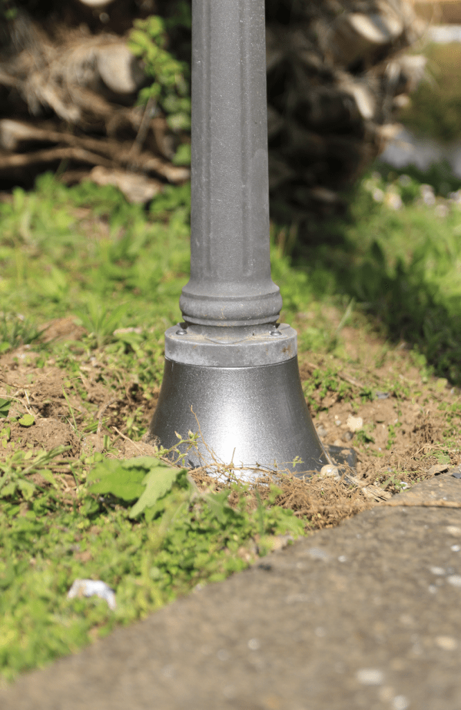
Nature is powerful, and not always in friendly ways. Climate and environmental agents like moisture, heat, and soil acidity can drastically affect the mechanical properties of materials, even those we think of as tough, like metal alloys.
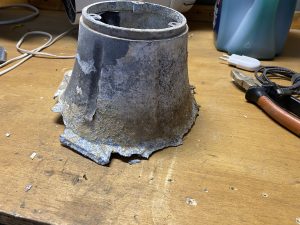
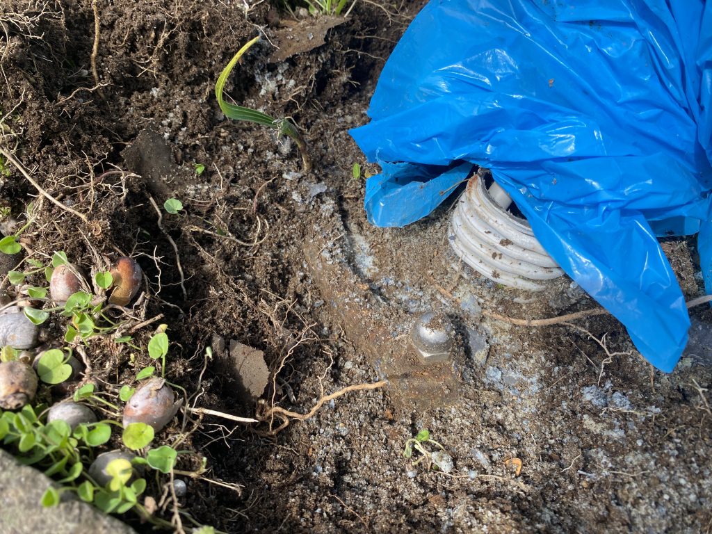
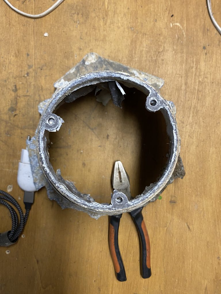
No, this isn’t about spacecraft or high-end medical devices. Let’s stay grounded — literally — in the garden. More specifically: the humble street lamp. The metal pole that once proudly stood upright has been slowly (but surely) degraded by a mix of humid soil, water, and scorching-hot sand. The alloy? Cheap and clearly not up to the challenge.
Now what? Should I buy a new lamp?
Sure, I could write a whole essay on throwaway culture and how everything’s harder to repair nowadays. But here’s the simple truth: the company that made the lamp no longer produces replacement parts.
So… what can we do? 3D print it.
It’s cheaper, faster (kind of), and gives us the freedom to customize and even improve the original design. Let’s dive into how I took this broken, rusted pole and gave it a new life — with a printer.
Table of Contents
Fixing the unfixable
Okay, despite being a backyard project and a little bit of fun, let’s approach this like proper engineers. That means solving the problem with a rigorous, functional mindset, not just duct tape and hope. So, what exactly do we need? We’re redesigning the lamp base, and it has to meet a few key requirements:
- The external size and shape must match the original, to fit neatly into the existing space and look coherent with the rest of the structure.
- The color should at least match the tone of the original, no weird patchwork aesthetics here.
- The bottom screw position is fixed, we can’t move the foundation, so our base has to adapt.
- The top screw holes need to align properly with the pole’s mounting holes, or the whole thing will twist and fail.
- An internal cavity is required to allow electrical cabling to pass through safely.
- It needs mechanical resistance, both to wind and to people who can’t resist leaning or falling into everything (why do you think this fall down?).
- It must withstand weather: rain, sun, heat, and cold, year-round.
This isn’t just a quick fix, it’s a small-scale, reverse-engineered, function-first redesign. With a little help from 3D printing, of course.
Let’s be honest, no engineering project feels real until we start throwing numbers around. We’ll get to mechanical strength calculations later, but for now let’s talk environment. The climate here is pretty standard: seasonal rain, warm summers, cold winters, nothing extreme. That means most 3D-printable materials are viable, except PLA, which is practically useless outdoors. It softens too easily under sunlight and heat, and we don’t want our lamp base to start sagging like a cooked noodle. The actual material selection is discussed in detail in the Durability section but we decided for PETG. For now, let’s focus on the most important constraints: the dimensions.
Design
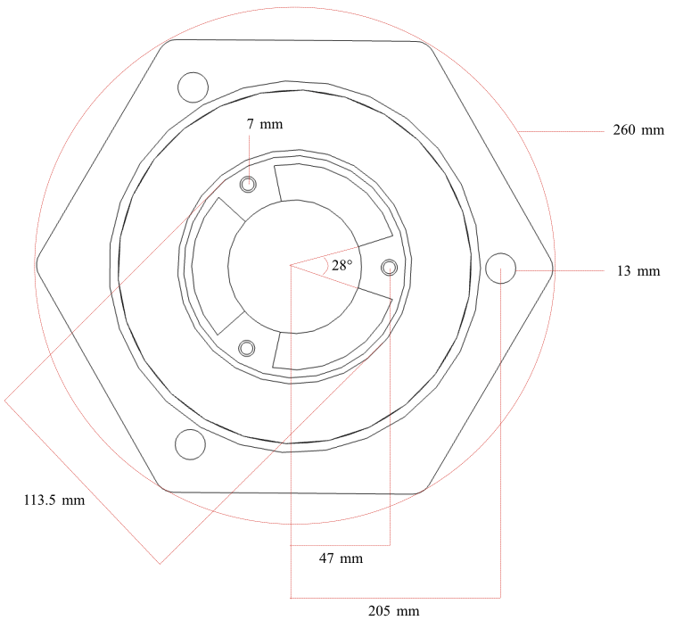
Dimensions are everything. In this case, most of what we need can be extracted from a photo — yes, it’s that DIY — but the key dimensional constraint is the base screw layout.
These three screws are arranged in a perfect equilateral triangle. Once we know the distance between any two screws, we can compute:
- The radius of the circumscribed circle
- The exact positions of all three screws
- And build all other geometry around that
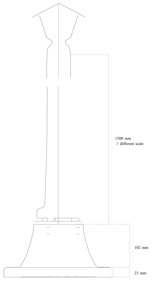
From there, we know the size of the base hexagon, which anchors the entire part. Then comes the connection to the lamp pole, which involves another set of three screws — this time positioned relative to the central hole. That interface is critical for alignment and structural stability. As for the external shape, the aesthetic curvature — we can extract that from a side photo and then adjust it to fit the real-world contour. Could we draw it manually in a CAD program? Sure. But do we want to?
Nope. Too Boring. Let’s Code It.
Computational CAD is a different paradigm from dragging shapes with a mouse in your favorite WYSIWYG CAD software. With computational CAD, you write code to define geometry. You don’t sketch lines, you define relationships, equations, and rules. It’s parametric. It’s repeatable. And once you get the hang of it, it’s actually more fun.
Let’s break it down:
- Define the screw triangle using simple trigonometry
- Extrude the base hexagon with thickness
- Cut a hole for the pole and define its mating surface
- Add the screw holes programmatically
- Model the outer contour curve with a mathematical function or image trace
All of it: done in code. Whether you’re using Mathematica, CadQuery, or even custom mesh generation in Unity or Python, this approach gives you full control, automation, and reproducibility.
Let’s walk through how we actually coded the geometry in the next section.
OpenCascade
OpenCascade is an open-source software development platform for 3D CAD, surface and solid modeling, visualization, and data exchange. It provides a robust set of C++ libraries for creating and manipulating complex geometric shapes, performing Boolean operations, meshing, and exporting/importing standard CAD formats like STEP and IGES. It can be integrated with Wolfram Mathematica.
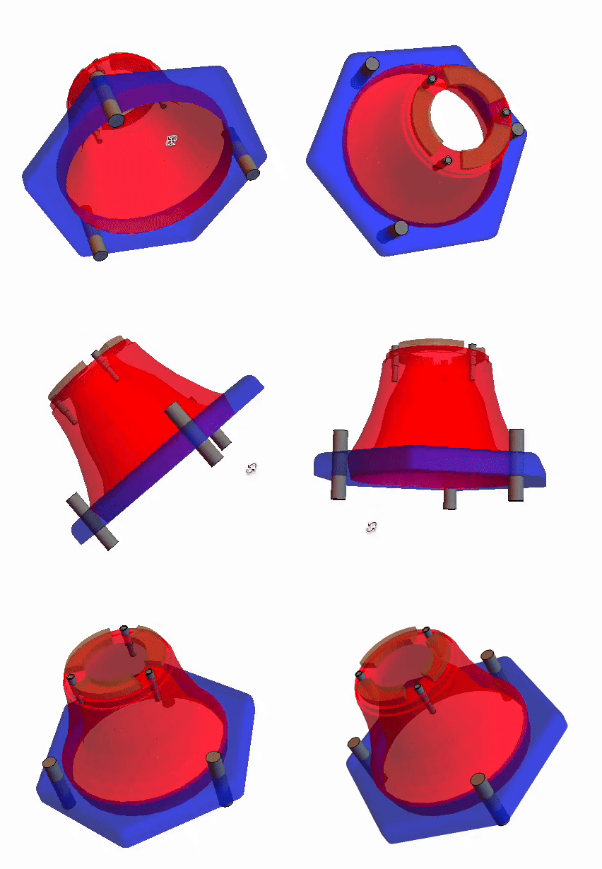
To generate the structure programmatically, we need to decompose it into several basic geometric components. As shown in the previous technical representation, the base can be interpreted as a large hexagon with a central hole. The main neck is modeled using a revolution geometry, while both the bottom and top holes are created by angularly spanningsegments of 120°, i.e., 360° divided into three sections. The final extrusion consists of an additional three geometries, each formed by splitting an annular disk.
The following figure highlights the different components: the base (blue), the main neck (red), the holes (gray), and the top extrusion (brown).
Let’s break down the structure by analyzing each component in detail.
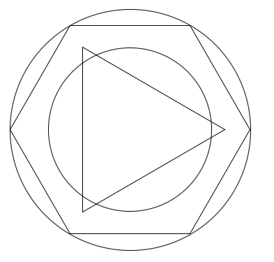
The dimensions can be obtained either by measuring the broken structure directly or by analyzing a photograph and rescaling it digitally. Since we aim to work with real-world, accurate dimensions, we begin by defining the parameters of a hexagon inscribed in a circle with a circumference of 260 mm.
scaleFactor = 10^-3;
hexDiam = 260;
internalDiamBase = 176;
holesDiam = 205;
It is interesting to note that the holes align with the vertices of an equivalent regular triangle, providing a helpful geometric reference.
Needs["OpenCascadeLink`"]
Needs["NDSolve`FEM`"]
With this setup, we can construct a planar hexagon, extrude it to a height of 23 mm, and then apply a fillet to round the top edges.
hBase = 23;
p2 = {0, 0, 0};
p1 = {0, 0, -hBase};
base2DShape = OpenCascadeShape[hex];
baseFilledPartial = OpenCascadeShapeLinearSweep[base2DShape, {p2, p1}];
list = Flatten@Table[{i, i + 1, i + 2}, {i, 1, 6*4, 4}]
baseFilledTotal = OpenCascadeShapeFillet[baseFilledPartial, 10, list]
hole2DShape = OpenCascadeShape[circDiff];
internalHoleShape = OpenCascadeShapeLinearSweep[hole2DShape, {p2, p1}];
When using OpenCascade, it’s important to explicitly specify the edges for the fillet operation. In this case, the relevant edges are simply edges 1, 2, and 3 of the six lateral faces — the fourth edge is excluded, as it corresponds to the bottom of the structure. Then we can remove the internal cylinder:
baseShape =
 OpenCascadeShapeDifference[baseFilledTotal, internalHoleShape]
Show[
(OpenCascadeShapeSurfaceMeshToBoundaryMesh[baseShape])[
"Wireframe"[
"MeshElementStyle" ->
Directive[Opacity[1], FaceForm[Brown], EdgeForm[]]]],
Graphics3D@Arrow[{p1, p2}]]The neck is modeled as a revolution geometry. Its cross-section is a trapezoidal-like plane shape, rotated around the vertical axis passing through the center. To define this section, we are constrained by the overall height, the top and bottom external radii, and the positions of the holes, so that the geometry can be used as a replacement for the original broken one. In other words, it must respect the external constraints imposed by the top lamp post, the concrete base, and the mounting screws.
h = 102;
topHeadR = 3;
topExternalRadius = topHeadR + 110.5/2;
topHeadH = 7.2;
topHolesSpan = 22;
l1 = Line[{{0, 0}, {holesDiam/2, 0}}];
l2 = Line[{{0, h}, {internalDiamBase/2, h}}];
shift = 16; (*shift=8;*) (*shift=4;*)
However, we are not constrained by the internal thickness, meaning we could theoretically fill the entire inner volume. As a starting point, we choose an average wall thickness (or shift) of 16 mm. This value will be further refined and optimized in the Finite Element Method (FEM) analysis section.
b2 = BSplineCurve[{
    p11 = {topExternalRadius, h},
    p11,
    {topExternalRadius*1.02, h*0.8},
    {topExternalRadius*1.2, h*0.4},
    {holesDiam/2, 0.05*h} - {10, 0} - {5, 0},
    p12 = {holesDiam/2, 0} - {10, 0}}, SplineKnots -> Automatic];
b1 = BSplineCurve[{
    p01 = {topExternalRadius - topHeadR - topHolesSpan, h},
    p01,
    p01 + {0, -topHolesSpan/2},
    {p01[[1]], h*0.6} + {topHolesSpan, 0},
    {p12[[1]] - 2.1 shift, h*0.1},
    p12 - {shift/2, shift/2},
    p02 = {internalDiamBase/2, -hBase}, p02
    }, SplineKnots -> Automatic];
The external profile, constrained at both the top and bottom points (shown in red), can be represented using a simple spline (in blue). The internal side, which is subject to fewer constraints, can be modeled with a second spline defined by a similar set of points (in green), shifted inward to represent the wall thickness. To form a closed profile suitable for revolution, the top and bottom edges (in black) must be enforced to ensure proper connection between the internal and external curves.
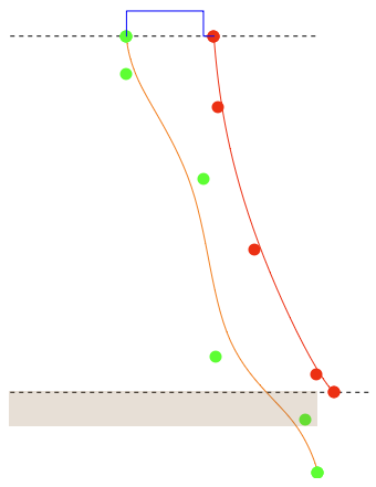
Graphics[{
  {Dashed, l1, l2},
  Red, b2, Orange, b1,
  {PointSize[0.03], Green, Point[b1[[1]]], Green, Point[{p01, p02}],
   Red, Point[b2[[1]]], Red, Point[b2[[1, 1]]], Point[b2[[1, -1]]]},
  {Brown, Opacity[0.2], Rectangle[{0, -10}, {internalDiamBase/2, 0}]},
  Blue,
  Line[{
    p11,
    ptop1 = {topExternalRadius - topHeadR, h},
    ptop2 = {topExternalRadius - topHeadR, h + topHeadH},
    ptop3 = {topExternalRadius - topHeadR - topHolesSpan,
      h + topHeadH},
    p01
    }]
  }]
We now need to combine the splines and straight segments into a closed shape using the appropriate OpenCascade function. Once the profile is closed, we can define the revolution sweep as follows:
externalShape = OpenCascadeShape[b2];
bottomLineShape = OpenCascadeShape[Line[{p12, p02}]];
internalShape = OpenCascadeShape[b1];
topLineShape = OpenCascadeShape[Line[{p01, ptop3, ptop2, ptop1, p11}]];

lineShape =
  OpenCascadeShapeUnion[{externalShape, bottomLineShape,
    internalShape, topLineShape}];
tf = RotationTransform[\[Pi]/2, {1, 0, 0}];
lineShapeRotated = OpenCascadeShapeTransformation[lineShape, tf];
sectionShape =
  OpenCascadeShapeFace[OpenCascadeShapeWire[lineShapeRotated]];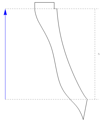
axis = {{0, 0, 0}, {0, 0, h}};
sweepShape =
 OpenCascadeShapeRotationalSweep[sectionShape, axis, 2 \[Pi]]
bmesh = OpenCascadeShapeSurfaceMeshToBoundaryMesh[sweepShape];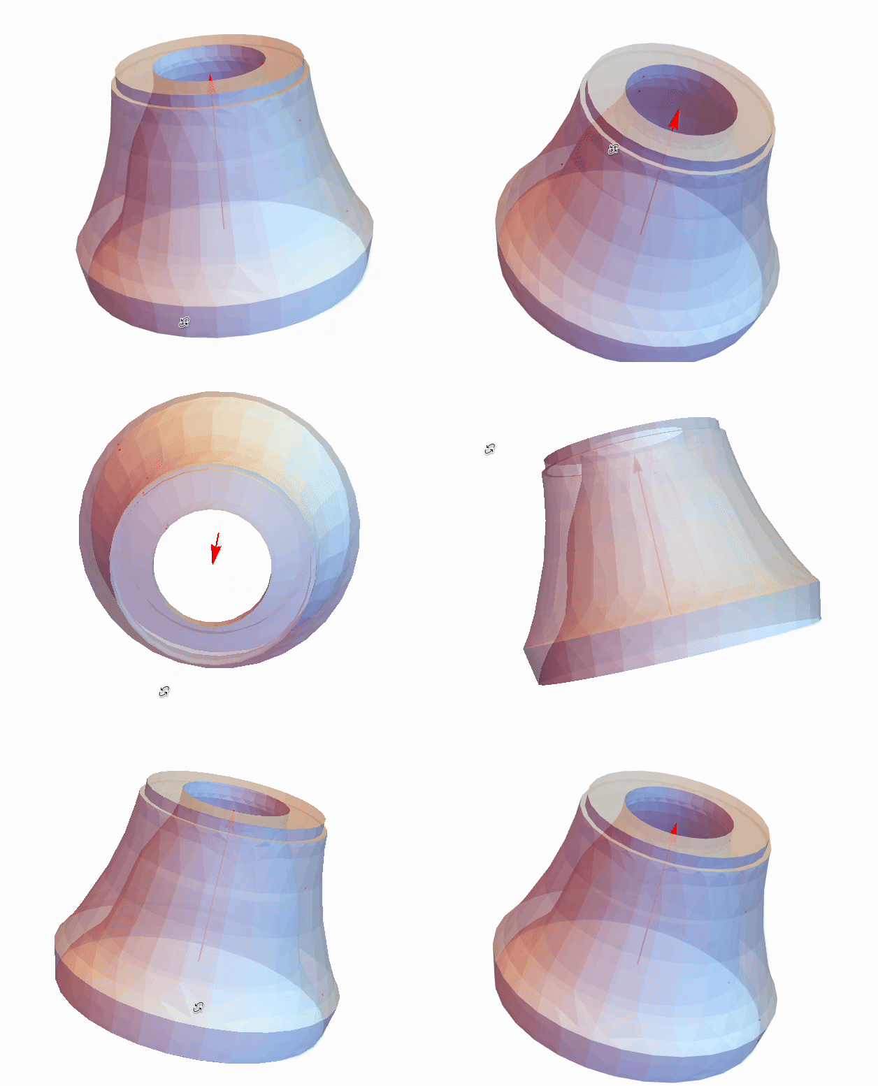
Show[Graphics3D[{{Red, Point[{0, #[[1]], #[[2]]}] & /@ b1[[1]]}, {Red,
     Thick, Arrow[axis]}}],
 bmesh["Wireframe"[
   "MeshElementStyle" ->
    Directive[Opacity[0.6], FaceForm[LightBlue], EdgeForm[]]]],
 Boxed -> False]
We can then combine the base and the neck using a boolean union operation to obtain a single, unified structure.
union = OpenCascadeShapeUnion[{sweepShape, baseShape}]
(bm = OpenCascadeShapeSurfaceMeshToBoundaryMesh[union])["Wireframe"]
topHolesInterDistance = 81.5;
topHolesH = topHolesInterDistance*Cos[30 Degree];
topHolesDistance = 2/3*topHolesH;Given the size of the holes, with the top ones designed to accommodate the insert and the bottom ones large enough for the base screws, we can model them as cylinders and subtract their geometry from the main body. As previously mentioned, the holes are angularly spaced by 120°, forming a regular triangular pattern.
pt = topHolesDistance*{Cos[# Degree], Sin[# Degree]} & /@ {0, 90 + 30, 180 + 60}bottomHoles = (Cylinder[{
{holesDiam/2*Cos[# Degree], holesDiam/2*Sin[# Degree], +hBase},
{holesDiam/2*Cos[# Degree], holesDiam/2*Sin[# Degree], -2 hBase}
}, bottomHolesDiam/2]) & /@ {0, 120, -120};
topHoles = (Cylinder[{
{topHolesDistance*Cos[# Degree], topHolesDistance*Sin[# Degree],
h + 2 topHeadH},
{topHolesDistance*Cos[# Degree], topHolesDistance*Sin[# Degree],
h + topHeadH - 14}
}, topHolesDiam/2]) & /@ {0, 120, -120};
topHolesSmaller = (Cylinder[{
{topHolesDistance*Cos[# Degree], topHolesDistance*Sin[# Degree],
h + 2 topHeadH},
{topHolesDistance*Cos[# Degree], topHolesDistance*Sin[# Degree],
h + topHeadH - 30}
}, 6/2]) & /@ {0, 120, -120};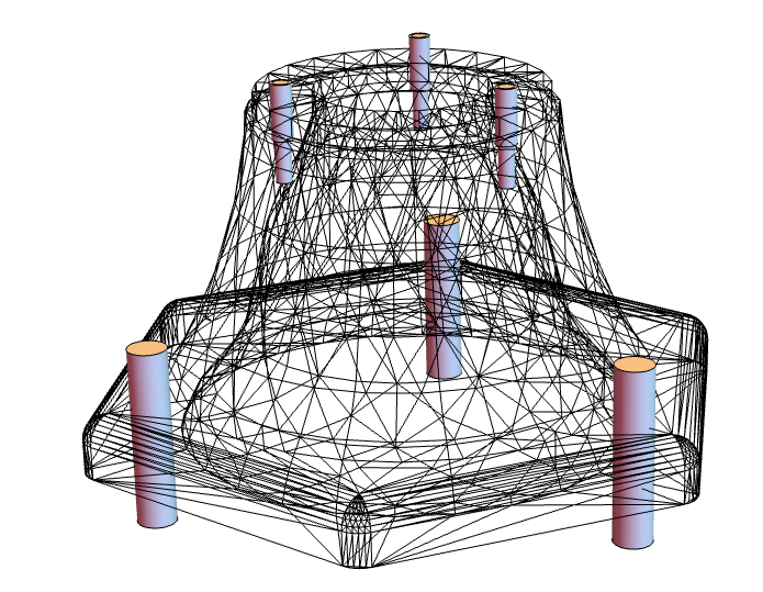
cylinders = Join[topHoles, bottomHoles, topHolesSmaller];
cylinderShapes = OpenCascadeShape[#] & /@ cylinders;
difference =
 OpenCascadeShapeDifference[union,
  OpenCascadeShapeUnion[cylinderShapes]]
(bm = OpenCascadeShapeSurfaceMeshToBoundaryMesh[
    difference])["Wireframe"]
The final top extrusion can be modeled as an annular section with the desired height, where a triangular segment is removed at the location of the holes. This results in a shape that matches the required geometry while maintaining clearance at those positions.
extraH = 7.8;
deltaThickness = 4;
extraSpace =
 OpenCascadeShapeDifference[
  OpenCascadeShape[
   Cylinder[{{0, 0, ptop2[[2]]}, {0, 0, ptop2[[2]] + extraH}},
    ptop2[[1]] - deltaThickness]],
  OpenCascadeShape[
   Cylinder[{{0, 0, ptop2[[2]]}, {0, 0, ptop2[[2]] + extraH}},
    ptop3[[1]]]]]
polys = Polygon[#] & /@ topHolesExtras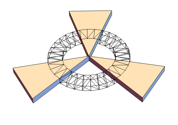
regs = RegionProduct[#,
    Line[{{ptop2[[2]]}, {ptop2[[2]] + extraH}}]] & /@ polys
cutterHoles = OpenCascadeShapeUnion[OpenCascadeShape[#] & /@ regs]
extrusion = OpenCascadeShapeDifference[extraSpace, cutterHoles];
extruted = OpenCascadeShapeUnion[difference, extrusion]
Material
We decided to use PETG due to its higher softening point compared to PLA. It offers good resistance to chemical substances, though it performs less well against weathering agents. From a durability standpoint, ASA would be a better choice. However, given its cost, up to three times higher, we opted for PETG.
The mechanical properties of 3D printed materials can vary significantly depending on print parameters such as infill pattern, infill density, layer orientation, and the number of perimeter or boundary layers. One of the key limitations of FDM-printed parts is the anisotropy introduced by the layer-by-layer fabrication process. This means that the strength of the material can differ depending on the direction of the applied load. Typically, intra-layer adhesion, the bonding within a single printed layer, is much stronger than inter-layer adhesion, which is where most failures occur, especially under tensile or flexural loading perpendicular to the layer lines. As a result, the fracture behavior of a printed part is strongly direction-dependent, and failure often initiates at weakly bonded interfaces.
To balance mechanical performance with material usage and print time, we opted for a triangular infill pattern at 50% density, which offers good structural efficiency. Additionally, we set 6 boundary (perimeter) layers to improve outer wall strength and enhance resistance to impacts and surface damage. This configuration ensures a strong shell to support loads while keeping the overall material usage below 500 grams per half, a practical constraint for both cost and print time without significantly compromising mechanical integrity.
3D print
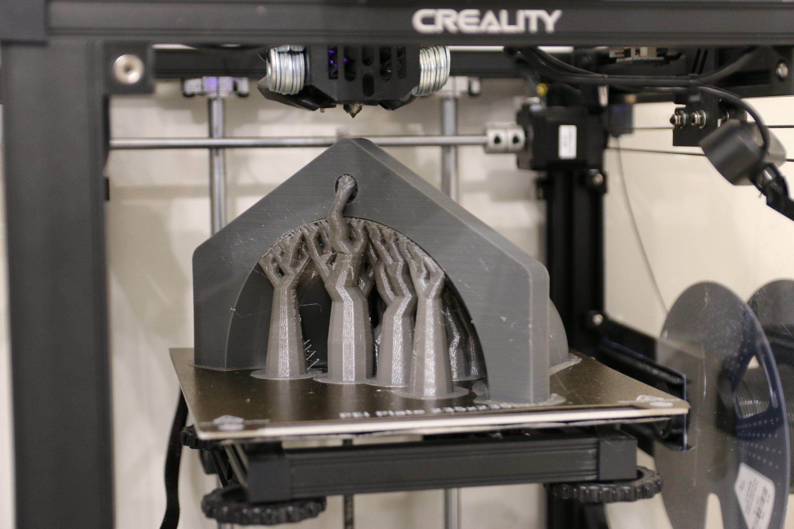
We can now divide the geometry into two segments to ensure it fits within the print bed dimensions. Additionally, printing in this orientation aligns the layer lines with the main axial loading direction of the geometry. This helps reduce the risk of delamination, especially in response to bending or deflection of the main pole. More details on this are discussed in the following section.
Set up a bounding box
xs = MinMax[bm["Coordinates"][[All, 1]]]
ys = MinMax[bm["Coordinates"][[All, 2]]]
zs = MinMax[bm["Coordinates"][[All, 3]]]
half = OpenCascadeShapeIntersection[extruted,
OpenCascadeShape[
Cuboid[{0, Min[xs[[1]], ys[[1]]], zs[[1]]},
1.1 {Max[xs[[2]], ys[[2]]], Max[xs[[2]], ys[[2]]], zs[[2]]}]]]
(bm2 = OpenCascadeShapeSurfaceMeshToBoundaryMesh[half,
"ShapeSurfaceMeshOptions" -> {"LinearDeflection" ->
0.0005}])["Wireframe"]half = OpenCascadeShapeDifference[extruted,
OpenCascadeShape[
Cuboid[{0, Min[xs[[1]], ys[[1]]], zs[[1]]},
1.1 {Max[xs[[2]], ys[[2]]], Max[xs[[2]], ys[[2]]], zs[[2]]}]]]
(bm2 = OpenCascadeShapeSurfaceMeshToBoundaryMesh[half,
"ShapeSurfaceMeshOptions" -> {"LinearDeflection" ->
0.0005}])["Wireframe"]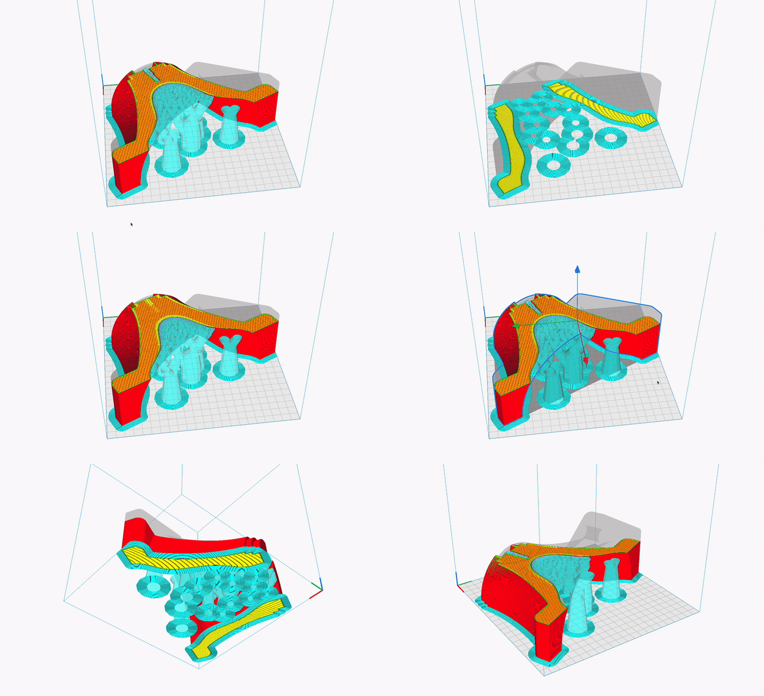
Threaded insert
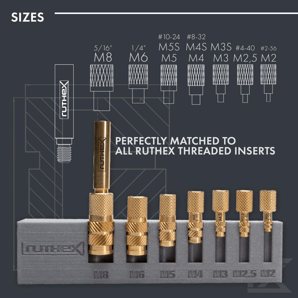
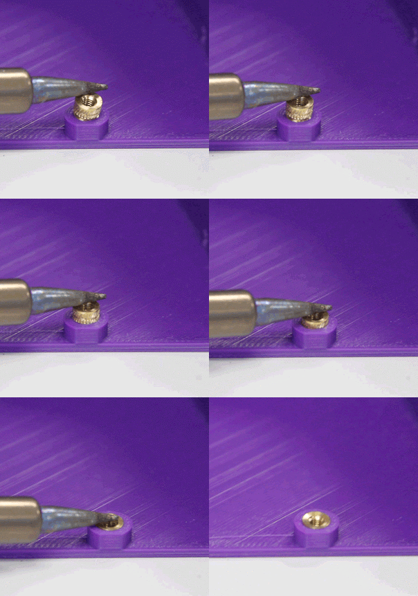
A threaded insert is a small metal component, usually made of brass, that is embedded into a 3D-printed part to provide strong, reusable threads for screws or bolts. They are commonly used in 3D printing because plastic threads can wear out or strip easily, especially under repeated use or high loads. Using threaded inserts improves durability, allows for better fastening, and gives the part a more professional, functional finish.
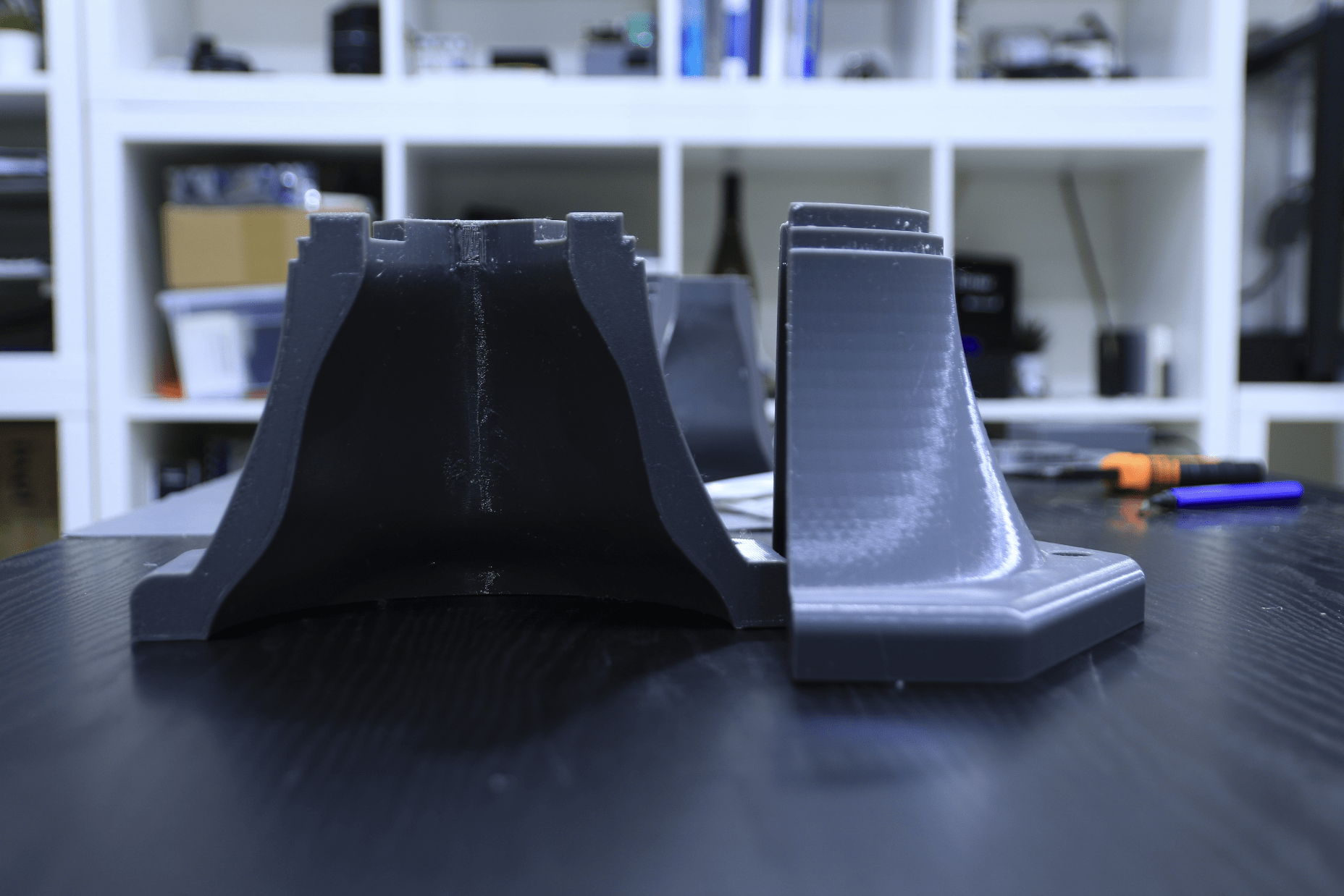
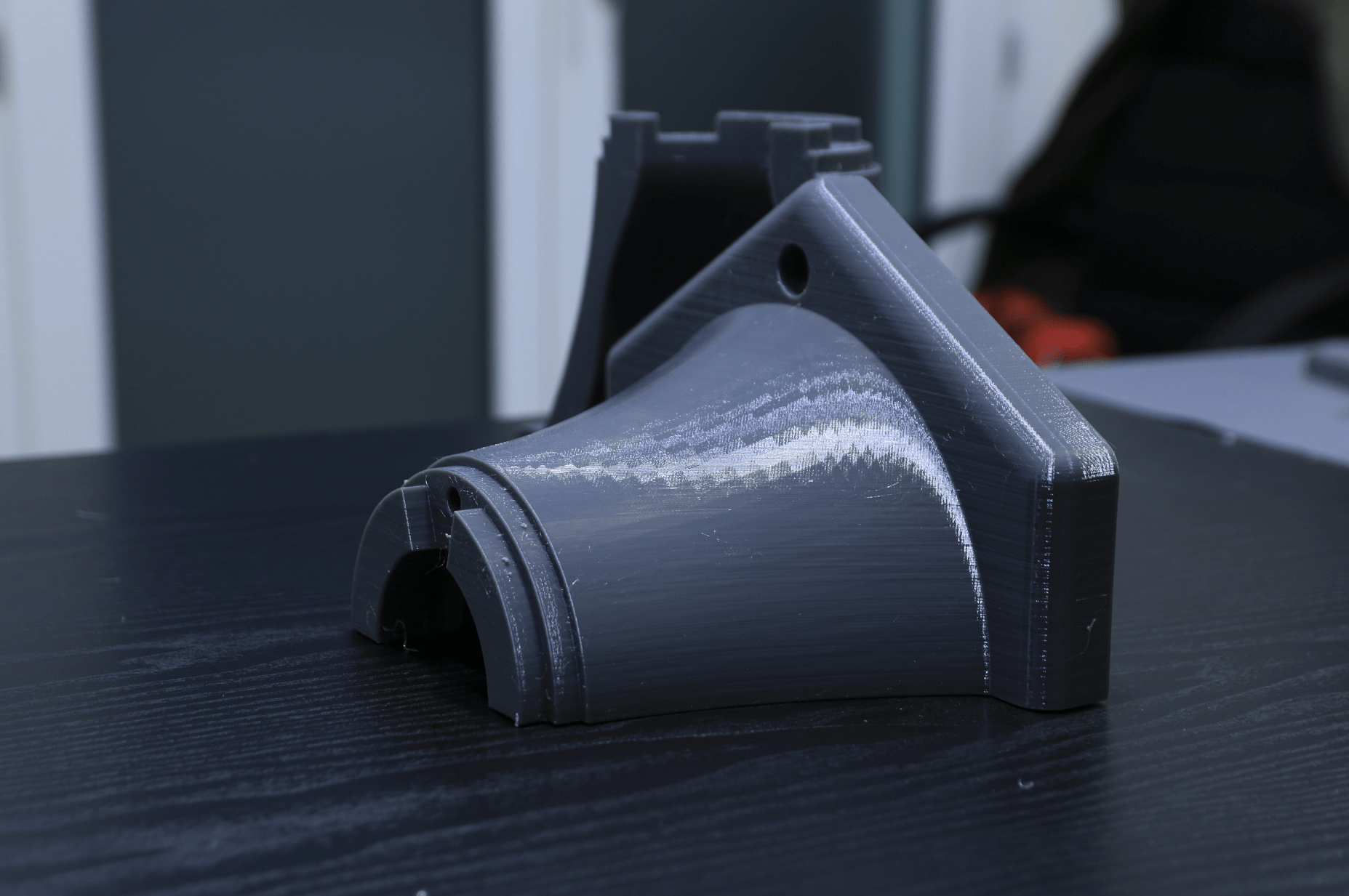
So yes, I went ahead and 3D printed it for real. What do you think?
FEM tools
Now, let’s try to understand what could happen to the material under loading. To analyze the stress and strain state, we need to define both the applied loads and the boundary conditions. Some choices are straightforward—such as using a linear elastic model for PETG with material properties provided by the filament manufacturer. Others, however, require a bit more consideration.
As a starting point, we can consider the failure load of a threaded insert, approximately 1200 Newton (see cnckitchen.com). This corresponds to a 10 kg load applied at 1.5 meters, which realistically represents the scenario of a person leaning on the pole. It serves as a reasonable baseline for analysis, and further safety considerations can be explored later.
Needs["NDSolve`FEM`"]Since the geometry was built directly in Mathematica, there’s no need for any complex import procedures. We can simply save and retrieve it using the .mx file format. However, it’s still important to ensure proper scaling: we need to verify the dimensions, and once the geometry is converted into a solid ElementMesh, we must rescale it back to millimeters to match real-world units.
bm = Import["/Users/alessandromastrofini/Downloads/Streetlight/bm.mx"]
meshTMP = ToElementMesh[bm, "MaxCellMeasure" -> 12]
mesh = ToElementMesh["Coordinates" -> 10^-3*meshTMP["Coordinates"],
  "MeshElements" -> meshTMP["MeshElements"]]
Show[mesh["Wireframe"], Axes -> True]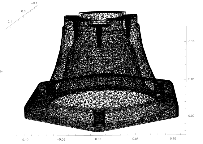
coords = mesh["Coordinates"];
bottom = Min[mesh["Coordinates"][[All, 3]]]
top = Max[mesh["Coordinates"][[All, 3]]]
Boundary conditions must be assigned to the top and bottom faces. These faces cannot move vertically, as the structure is supported by the concrete base. Additionally, the bottom holes can be considered fixed, due to the constraint imposed by the screws anchoring the part.
As for the top faces, we can model a bending moment. This can be represented by applying a vertical load along the Z-axis, where half of the face area is in compression (pushing downward), and the other half in tension, particularly in the regions around the insert holes, simulating the pulling effect of the screw under load.
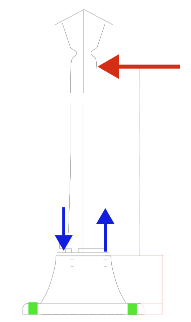
External load (red), reported load (blue) and fixed point (green)
Are we sure about the external load?
Given the required load distribution, we can take advantage of the geometrical properties of the structure. Specifically, the surface region of interest can be approximated as a half-annulus with inner and outer radii r1 and r2 . The applied load can be modeled as a distributed force, defined as follows, where minX refers to the coordinate of the point farthest from the origin along the x-axis, based on the current orientation.
Here, F represents the magnitude of the distributed load. According to mechanical equilibrium, the resulting momentfrom this distribution must be equivalent to the total force applied (i.e., the integral of the distributed load over the region).
This setup is intended to replicate the moment generated by a 1200 N pulling force applied at the opposite insert hole. Numerically:
minLoadedX = Min[coords[[tt]][[All, 1]]]
distrLoad = F*x/minLoadedX;
insertFailureLoad = 1200;
noInserts = 3;
tensileLoad = noInserts*insertFailureLoad;
M = tensileLoad * rH;
totalMoment =
 Integrate[distrLoad x, {x, y} \[Element] \[ScriptCapitalR]]
\[ScriptCapitalR] = Region[Annulus[{0, 0}, {r1, r2}, {Pi/2, 3 Pi/2}]]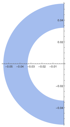
sol = Solve[totalMoment == M, F]
loadFun[x_] := (distrLoad /. sol)[[1]]
Which corresponds to:
It’s worth noting that the same rotational equilibrium corresponds to an equivalent load applied to the lamp pole at a distance of 1.5 meters from the base — roughly the effect of a 10 kg weight, similar to a person leaning on the pole.
To assign the external load, we need to define Boolean conditions based on the position of the nodes.
For the insert region, nodes can be selected using the equation of a circle, defined by its center and radius.
topHolesCenters =
  10^-3 47.05404693895449`*{Cos[# Degree], Sin[# Degree]} & /@ {0,
    90 + 30, 180 + 60};
topHolesRadius = 8*10^-3/2;
loadedHoleNodesCondition =
 (x - topHolesCenters[[1, 1]])^2 + (y - topHolesCenters[[1, 2]])^2 <=
topHolesRadius^2For the top face under compression, we need to select nodes that satisfy all the following criteria:
- lie on the top surface,
- have a negative x-coordinate
- are located within the region corresponding to the top surface minus the thickness of the top extrusion, restricted to the relevant angular sectors
To do that we can simply assign the conditions bases on the lowest z and it will recognize to propers surface:
extraH = 10^-3*7.8;
topBCs = z >= (top - extraH - 10^-5) && x <= 0 + 10^-5;
The equilibrium equations describe the relationship between the body force density F [N/m³] and the resulting stress σ [Pa]. The dynamic equilibrium equation is expressed as:
where ρ is the mass density and u is the displacement vector. The force density F may act throughout the volume of the body or be applied on its boundary. The kinematic equations link the displacement field u to the strain tensor ε, which quantifies the relative displacement between points within the material. Strain captures how the shape or size of a body changes under loading.
To connect the kinematic and equilibrium equations, we use constitutive relations, which define the material’s response. Assuming a linearly elastic material, the constitutive law is:
where C is the stifness matrix, a material constant representing stiffness. Most metals and many polymers behave elastically under small strains, making this linear model widely applicable.
For the assumed PETG material, a typical value for Young’s modulus is approximately 2.9 GPa, though it can vary by up to 50%, depending on factors such as infill percentage and print parameters. See Mohamad et al and sunlu.com for details.
The physics of the problem is governed by a set of Partial Differential Equations (PDEs), which are formulated and assembled in the following section using Mathematica’s built-in Solid Mechanics Finite Element Method (FEM) library.
Now we can assemble the system of equations and use NDSolve to solve the problem numerically:
A = NIntegrate[1, {x, y} \[Element] \[ScriptCapitalR]];

pde = {
   SolidMechanicsPDEComponent[vars,pars] ==(SolidBoundaryLoadValue[topBCs, vars,
       pars, <|"Force" -> {0, 0, A*loadFun[x]}|>] +
      SolidBoundaryLoadValue[loadedHoleNodesCondition, vars,
       pars, <|"Force" -> {0, 0, tensileLoad}|>]
     ),

   SolidDisplacementCondition[z == bottom, vars, pars,<|"Displacement" -> {None, None, 0}|>],
   SolidFixedCondition[bottomHolesNodesCondition, vars, pars]
   };
FEM solution:
displ = NDSolveValue[pde, {u[x, y, z], v[x, y, z], w[x, y, z]}, {x, y, z} \[Element] mesh];
We can compare four different thickness values for the main neck. This comparison will provide useful insights and help identify the best compromise between mechanical strength, material cost and usage, printing orientation, and risk of failure, by varying the shift parameter.
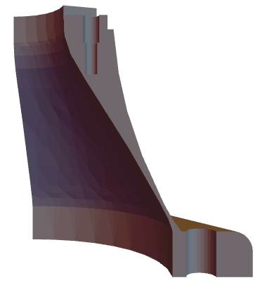
4 mm
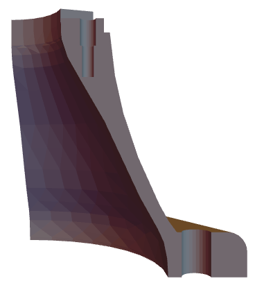
8 mm
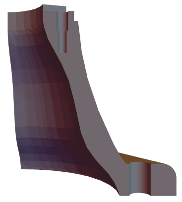
16 mm
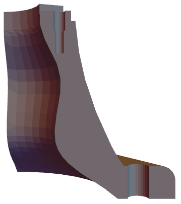
28 mm
By comparing the maximum stress values across the different structural configurations, we can identify the most efficient design, one that allows us to reduce material usage as much as possible, while still maintaining a safe distance from the material’s failure threshold. This approach not only optimizes the structure from a mechanical perspective but also contributes to cost savings and improved printability, without compromising overall reliability and performance.
3D Von Mises stress [MPa] plot for the 16mm one on half structure. The mesh is deformed with a x100 factor.
Stress and failure
As expected, increasing the wall thickness leads to a reduction in peak stress within the structure. However, an interesting observation arises in the case of thinner geometries: rather than experiencing pure compression, the material begins to exhibit flexural behavior. This shift can significantly increase the risk of failure—especially in materials like PETG, which may have an inter-layer strength as low as 10–15% of the intra-layer strength. In such cases, delaminationbecomes a critical concern, particularly under bending loads. The failure limit of the PETG is around the 5-10% of strains resulting approximately in a stress value of 30-150 MPa.
3D Von Mises stress [MPa] plot for the 4mm one, where the value exceeds the 10% of the failure one. The mesh is deformed with a x100 factor.
3D Von Mises stress [MPa] plot for the 8mm one, where the value exceeds the 10% of the failure one. The mesh is deformed with a x100 factor.
On the other hand, the thickest configuration provides excellent mechanical resistance but results in excessive filament usage, which may not be practical or efficient for production. A reasonable compromise could be found in the 8 mm to 16 mm thickness range. Further analysis could involve adjusting the safety factor closer to PETG’s actual failure threshold to select the most material-efficient design that still ensures structural reliability.
3D Von Mises stress [MPa] plot for the 16mm one, where the value exceeds the 10% of the failure one. The mesh is deformed with a x100 factor.
3D Von Mises stress [MPa] plot for the 28mm one, where the value exceeds the 10% of the failure one. The mesh is deformed with a x100 factor.
The 16 mm option appears to be a good compromise.
Safety factor based on the 50% limit in term of tensile ultimate strength.
Safety factor based on the 50% limit in term of tensile ultimate strength.
As observed, the highest stress concentrations are located near the insert regions. This is expected and acceptable, as the insert–PETG interface is likely to fail before the structural base itself collapses. However, it’s important to consider that impact loads, such as someone suddenly leaning or bumping into the structure, can reach values up to 10 times higherthan the proposed static load. This significantly increases the risk of localized failure, particularly in weaker areas like the insert interface.
Given the relatively low cost of 3D printing filament, selecting a 16 mm thickness is a practical and safe choice, as it consistently provides a generous safety margin. Moreover, the component may be subjected to various forms of external stress, including impacts from garden tools or long-term environmental degradation due to exposure to sun, moisture, or temperature fluctuations. In this context, a thicker wall not only improves structural strength but also enhances the durability and resilience of the part in real-world conditions.
Durability
To improve its resistance to UV exposure, we chose to paint the part. First, we applied a plastic adhesion promoter, followed by a spray paint designed to mimic a cast iron finish.
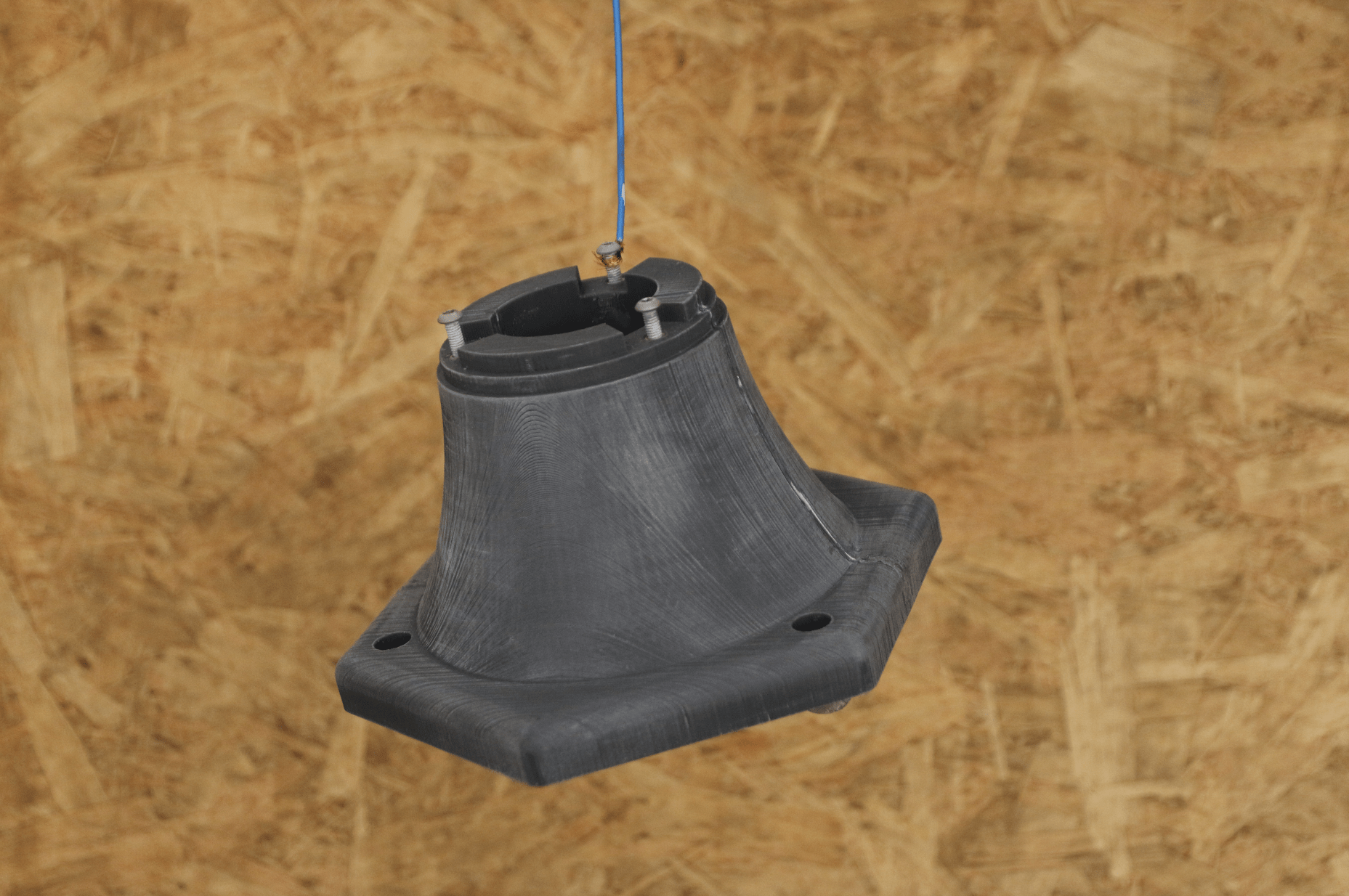
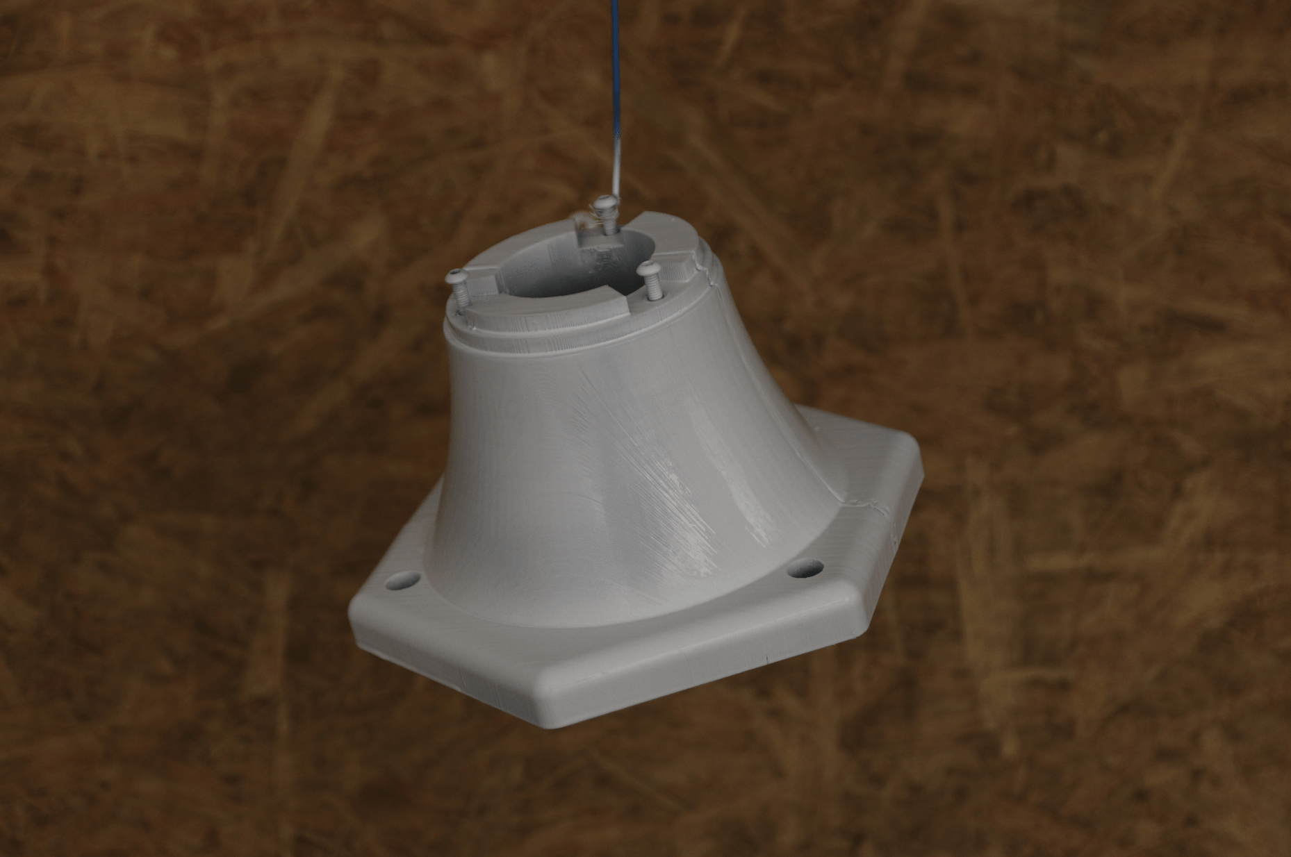
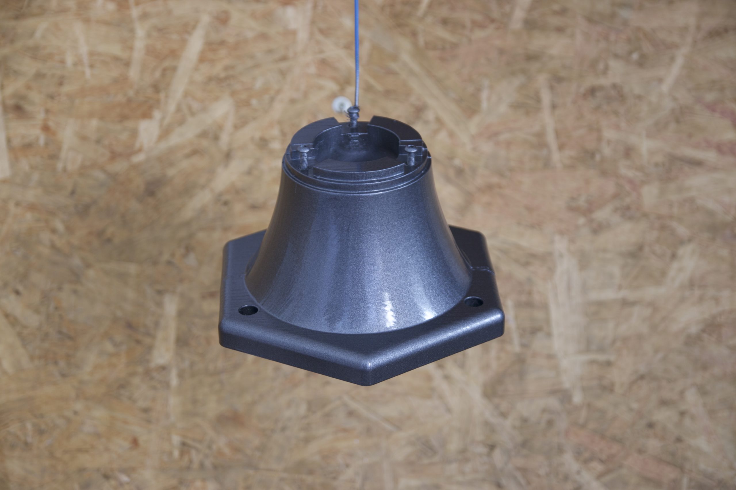
The final result looks clean and well integrated. Hopefully, it will also hold up well over time.